【Python数据分析案例】（十九）——预测泰坦尼克号乘员的生存(机器学习全流程)

网盘截屏

▶全部源码和数据，请点击“支付下载”获取！支付后无网盘链接，请联系客服QQ：3345172409或1919588043（微信同号）☺

导读

上一篇数据分析案例是回归问题，本次案例带来分类问题的 机器学习案例。这个数据集比上个案例更小、更简单，代码也不复杂，新手都可以学一学。

背景分析

预测乘客是否存活下来
泰坦尼克号是数据科学机器学习领域很经典的数据集，在统计学里面也有很多案例，比如拟合优度检验，方差分析等等。其背景就是当年泰坦尼克号上那么多人，灾难发生后，有人生存有人死亡，而且每个人都有很多不同的特征，比如性别，年龄，船仓等级，登船地点等等…..根据这些特征，我们可以预测乘客是否存活下来。

存活是1，死亡是0，响应变量为两种取值，所以这是一个分类问题。

数据收集和读取

从kaggle上下载泰坦尼克号的数据¶
kaggle是国际很有名的数据科学竞赛平台，上面有很多比赛，也有很多数据集，大家可以注册一个账号去看看。下面是泰坦尼克号的项目链接。

Titanic – Machine Learning from Disaster | Kaggle

当然下载数据要登陆账号，而注册账号需要翻墙……如果不方便弄个vpn，但需要泰坦尼克号数据集，可以评论找博主要。

导入数据分析常用包

import numpy as np
import pandas as pd
import matplotlib.pyplot as plt
import seaborn as sns

读取数据，分训练集和测试集读取

data=pd.read_csv('train.csv')
data2=pd.read_csv('test.csv')

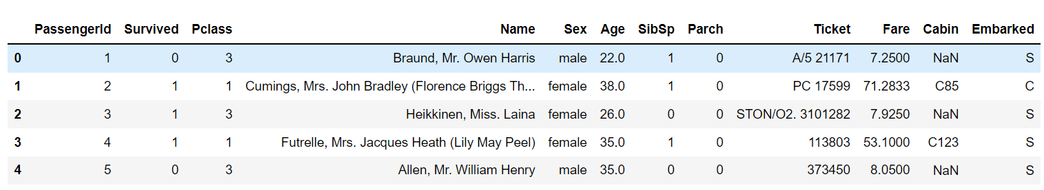
展示训练集前五行数据

data.head(5)

展示测试集前五行数据

data2.head(5)

可以看到第一列是乘客的编号。我们的响应变量是Survived，即乘客是否存活，但是测试集是没有这一列的，因为需要我们预测。

后面都是特征变量，乘客的特征：船舱等级、姓名，性别，年龄，子女个数，亲戚个数，船费、登船地点等等¶

数据清洗和整理

查看数据信息¶

data.info()
data2.info()

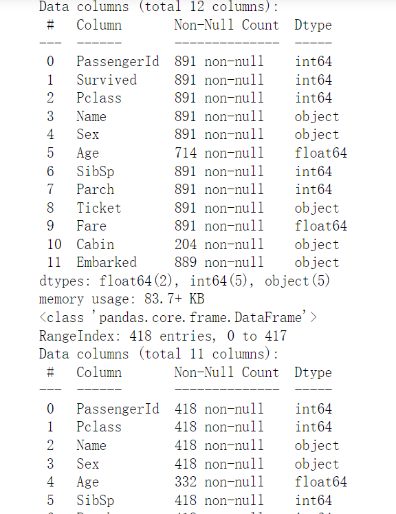
这里没有截完。可以看到训练集891条数据，测试集418条数据。还有的列是没有这么多的，因为存在缺失值。

数据存在一定的缺失值，进一步画图看缺失值

画图看缺失值

import missingno as msno
%matplotlib inline
msno.matrix(data)

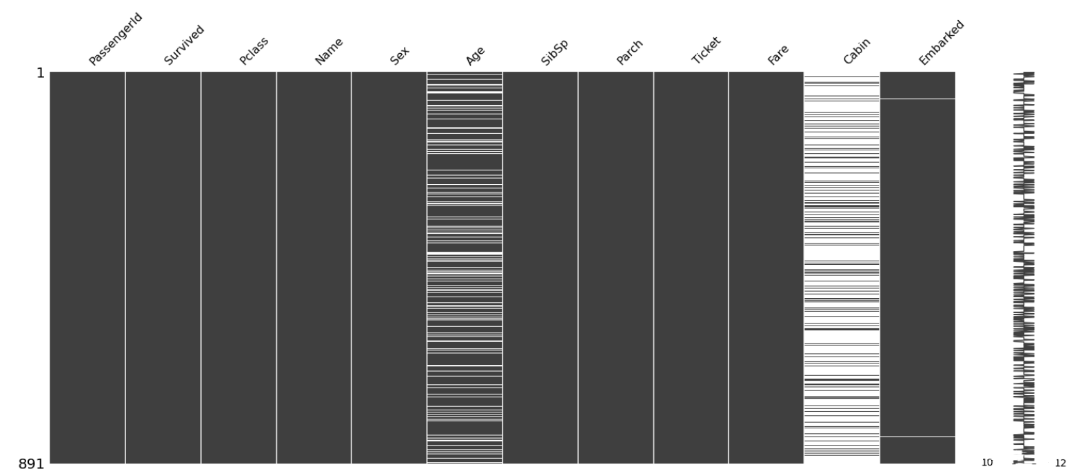
测试集也类似，不展示了。

这个图就是黑色的位置表示有数据，白色表示数据的缺失，可以看到cabin这一列缺失值很多，age年龄缺失值也较多。

数据清洗
特征选择
下面删除一些不需要的变量，比如乘客编号、名字、船票编号等等，还有缺失值很多的Cabin变量

y=data['Survived']
data.drop ('Survived',axis=1, inplace=True)

data.drop ('PassengerId',axis=1, inplace=True)
data.drop ('Name',axis=1, inplace=True)
data.drop ('Ticket',axis=1, inplace=True)
data.drop ('Cabin',axis=1, inplace=True)

ID=data2['PassengerId']
data2.drop ('PassengerId',axis=1, inplace=True)
data2.drop ('Name',axis=1, inplace=True)
data2.drop ('Ticket',axis=1, inplace=True)
data2.drop ('Cabin',axis=1, inplace=True)

缺失值填充
对年龄等缺失值位置进行填充，采用中位数填充

data['Age'].fillna(data.Age.median(), inplace=True)
data['Embarked'].fillna(method='pad',axis=0,inplace=True)

data2['Age'].fillna(data2.Age.median(), inplace=True)
data2['Fare'].fillna(method='pad',axis=0,inplace=True)

分类型数据转化
将文本型的分类数据映射为数值型数据，例如男：0，女：1

d1={'male':0,'female':1}
d2={'S':1,'C':2,'Q':3}

data['Sex']=data['Sex'].map(d1)
data['Embarked']=data['Embarked'].map(d2)

data2['Sex']=data2['Sex'].map(d1)
data2['Embarked']=data2['Embarked'].map(d2)

特征工程
整理好后查看数据信息
将数据赋值给X表示为响应变量

X=data.copy()
test=data2.copy()
X.info()
test.info()

可以看到没有缺失值了。

画图查看训练集和测试集的变量分布情况

dist_cols = 4
dist_rows = len(data2.columns)
plt.figure(figsize=(4 * dist_cols, 4 * dist_rows))
i = 1
for col in data2.columns:
ax = plt.subplot(dist_rows, dist_cols, i)
ax = sns.kdeplot(data[col], color="Red", shade=True)
ax = sns.kdeplot(data2[col], color="Blue", shade=True)
ax.set_xlabel(col)
ax.set_ylabel("Frequency")
ax = ax.legend(["train", "test"])
i += 1
plt.show()

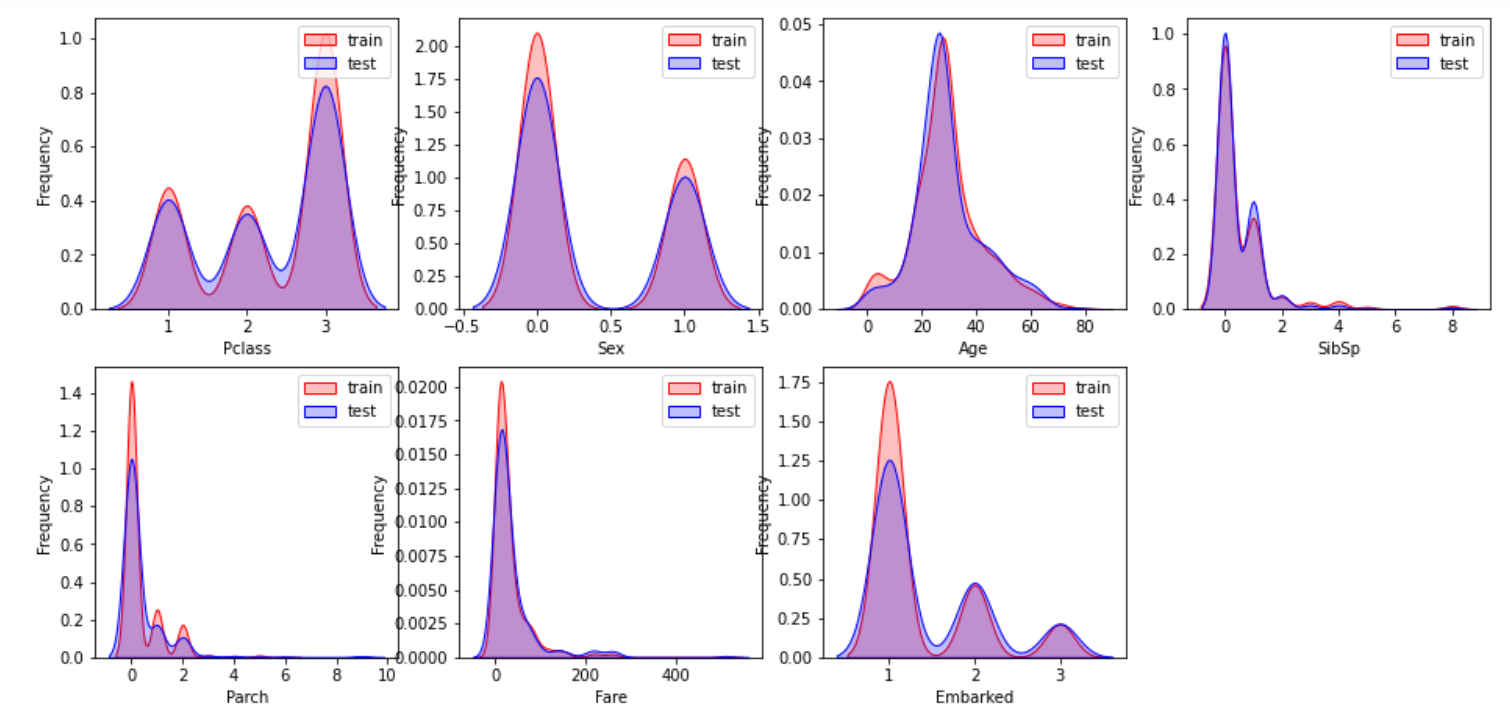
训练集和测试集的数据分布还是很一致的。

查看相关系数矩阵

corr = plt.subplots(figsize = (8,6))
corr= sns.heatmap(data.corr(method='spearman'),annot=True,square=True)

每个变量之间的相关性还是不太高的，只有船舱等级和船费相关性是负数，还比较高，这也是理所当然的。给的钱越多当然坐更好的船仓。

测试集也差不多就不展示了。

建模与优化

开始机器学习！

划分训练集和验证集

from sklearn.model_selection import train_test_split
X_train,X_val,y_train,y_val=train_test_split(X,y,test_size=0.2,stratify=y,random_state=0)

这里是二八开，80%数据训练，20%数据验证。

数据标准化

from sklearn.preprocessing import StandardScaler
scaler = StandardScaler()
scaler.fit(X_train)
X_train_s = scaler.transform(X_train)
X_val_s = scaler.transform(X_val)
test_s=scaler.transform(test)

构建自适应提升模型
我们先用一个简单的集成模型来验证一下精度

#自适应提升
from sklearn.ensemble import AdaBoostClassifier
model0 = AdaBoostClassifier(n_estimators=100,random_state=77)
model0.fit(X_train_s, y_train)
model0.score(X_val_s, y_val)

模型在验证集上的精度为0.7988，还可以。

模型运用——预测

存储预测结果
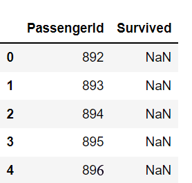
#准备存储预测结果表格

df = pd.DataFrame(columns=['PassengerId','Survived'])
df['PassengerId']=ID
df.head()

对测试集上的数据预测，然后结果填入上述表格中储存就行

pred = model0.predict(test_s)
df[‘Survived’]=pred
df.to_csv(‘predict_result__AdaBoost.csv’,index=False)

模型选择和优化

模型选择
采用十种模型，分别看谁在验证集的精度高

from sklearn.linear_model import LogisticRegression
from sklearn.discriminant_analysis import LinearDiscriminantAnalysis
from sklearn.neighbors import KNeighborsClassifier
from sklearn.tree import DecisionTreeClassifier
from sklearn.ensemble import RandomForestClassifier
from sklearn.ensemble import GradientBoostingClassifier
from xgboost.sklearn import XGBClassifier
from sklearn.svm import SVC
from sklearn.neural_network import MLPClassifier
#逻辑回归
model1 = LogisticRegression(C=1e10)

#线性判别分析
model2 = LinearDiscriminantAnalysis()

#K近邻
model3 = KNeighborsClassifier(n_neighbors=10)

#决策树
model4 = DecisionTreeClassifier(random_state=77)

#随机森林
model5= RandomForestClassifier(n_estimators=1000, max_features='sqrt',random_state=10)

#梯度提升
model6 = GradientBoostingClassifier(random_state=123)

#极端梯度提升
model7 = XGBClassifier(eval_metric=['logloss','auc','error'],n_estimators=1000,
colsample_bytree=0.8,learning_rate=0.1,random_state=77)

#支持向量机
model8 = SVC(kernel="rbf", random_state=77)

#神经网络
model9 = MLPClassifier(hidden_layer_sizes=(16,8), random_state=77, max_iter=10000)

model_list=[model1,model2,model3,model4,model5,model6,model7,model8,model9]
model_name=['逻辑回归','线性判别','K近邻','决策树','随机森林','梯度提升','极端梯度提升','支持向量机','神经网络']

将精度打印出来，预测结果都存储下来

for i in range(9):
model_C=model_list[i]
name=model_name[i]
model_C.fit(X_train_s, y_train)
s=model_C.score(X_val_s, y_val)
print(name+'方法在验证集的准确率为：'+str(s))
pred = model_C.predict(test_s)
df['Survived']=pred
csv_name=name+'的预测结果.csv'
df.to_csv(csv_name,index=False)

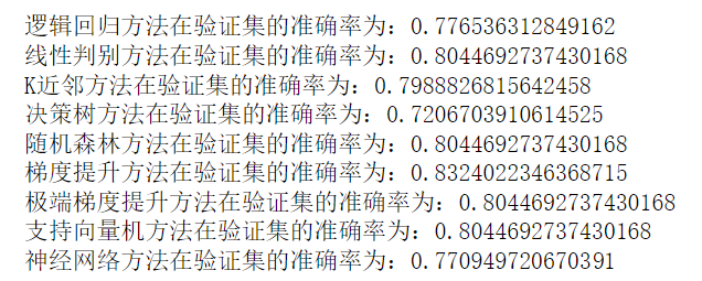
发现梯度提升方法精度最高，进一步优化

模型优化

模型再继续优化就是调整超参数，这里利用K折交叉验证搜索最优超参数

from sklearn.model_selection import KFold, StratifiedKFold
from sklearn.model_selection import GridSearchCV

我们对max_depth’和 ‘learning_rate这两个超参数进行网格化搜索。当然也有很多别的参数也可以搜索，可以多试试。

# Choose best hyperparameters by RandomizedSearchCV
param_distributions = {'max_depth': range(1, 10), 'learning_rate': np.linspace(0.1,0.5,5 )}
kfold = StratifiedKFold(n_splits=10, shuffle=True, random_state=1)

model = GridSearchCV(estimator=GradientBoostingClassifier(n_estimators=300,random_state=123),
param_grid=param_distributions, cv=kfold)
model.fit(X_train_s, y_train)
model.best_params_

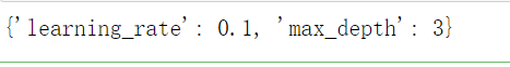
可以看到最优参数是0.1和3

此时模型的精度为

model = model.best_estimator_
model.score(X_val_s, y_val)

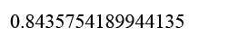
模型精度进一步提升到0.84357，然后储存结果

pred = model.predict(test_s)
df['Survived']=pred
df.to_csv('调参后的梯度提升预测结果.csv',index=False)

这样就做完啦，可以把储存出来的文件提交到kaggle上看自己的模型精度的排名了！

八、模型评价

我们可以进一步看看是哪个特征对于是否存活的预测起到的重要作用。

得到特征变量的重要性排序图

sorted_index = model.feature_importances_.argsort()
plt.barh(range(X.shape[1]), model.feature_importances_[sorted_index])
plt.yticks(np.arange(X.shape[1]), X.columns[sorted_index])
plt.xlabel('Feature Importance')
plt.ylabel('Feature')
plt.title('Gradient Boosting')

我们可以看到性别对于是否存活起到了重要的作用。

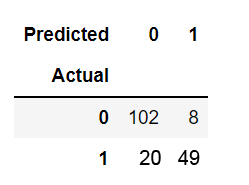
画出混淆矩阵

# Prediction Performance 
#prob = model.predict_proba(X_test)
pred = model.predict(X_val_s)
table = pd.crosstab(y_val, pred, rownames=['Actual'], colnames=['Predicted'])
table

AUC图

计算AUC指标，并画图

from sklearn.metrics import plot_roc_curve
plot_roc_curve(model, X_val_s, y_val)
x = np.linspace(0, 1, 100)
plt.plot(x, x, 'k--', linewidth=1)

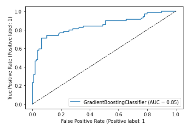
AUC为1最好，我们模型为0.85，也很不错